Yes. The data files you upload for analysis as well as any analysis results, are not downloaded or examined in any way by
the administrators, unless required for system maintenance and troubleshooting. All files will be deleted automatically after
72 hours, and no archives or backups are kept unless you have registered an account and saved the analysis.
You are advised to download your results immediately after performing an analysis.
NetworkAnalyst accepts data from 17 species, in the following formats:
List(s) of genes or proteins: one or more lists of gene or protein IDs with optional expression profiles (i.e. fold changes).
Each gene should be in a row. Please refer to our example data for more details.
Network file: users can upload network files generated with a different software to perform network visualization in
NetworkAnalyst. More details on network file formats are provided in the corresponding questions below.
NetworkAnalyst support four different types of files (.sif, .txt(edge list), .graphml and .json).
Please click on the following links to see example files supported:
The goal of network construction is to generate a clear visualization of the biological context of the genes of interest.
This includes capturing relevant biological pathways and molecules (TFs, drugs, chemicals) that interact with the gene list,
as well as important connections between them. For a small gene list (< 100), this is accomplished by adding a
substantial number of interacting nodes from the underlaying databases. For a large gene list (> 1000), there are likely enough
biological interactions within the uploaded list and so network construction is focused on pruning nodes and edges
to reduce complexity to more effectively interpret the most critical connections.
The networks are generated by first mapping the significant genes/proteins to the selected
underlying database. A search algorithm is then performed to identify proteins that directly interact with
the uploaded genes/proteins ("seeds"). The seeds and their interaction partners are returned to
build the subnetworks.
This approach will typically return one giant subnetwork ("continent") with multiple smaller ones ("islands").
Most subsequent analysis is performed on the continent. Note, networks with less than 3 nodes will be excluded.
To perform integration, select more than databases in "Network Selection" page. There exists two integration options
Union: create multi-modal networks by creating a network that is the union of first-order networks of selected databases.
Intersection: identify the share portion of multiple first-order networks. A useful use case is to integrate tissue specific coexpression with generic PPI.
The visualization is actually limited by the performance of users' computers and screen resolutions.
Too many nodes will make the network too dense to visualize and the computer slow to respond.
We recommend limiting the total number of nodes to between 200 ~ 2000 for the best experience.
For very large networks, please make sure you have a decent computer equipped with a modern browser
(we recommend the latest Google Chrome).
When there are too few seed genes, the resulting network will be too simplified to identify themes in the biological context
of you genes of interest. There are two main solutions here:
Expand your search of the underlaying database by using a Second-order Network;
Increase the input genes by using smaller fold change and/or larger p value cutoffs.
When there are a large number of significant genes or seed proteins, the resulting networks will be
too large and complex for effective visualization and interpretation. There are four possible solutions here:
Reduce the networks using direct connections between seed proteins Zero-order Network;
Trim the networks to keep only seeds and their connecting nodes using Minimum Network
or Steiner Forest Network;
Filter the networks using the Degree Filter or Betweenness Filter;
Reduce the input genes by using larger fold change and/or smaller p value cutoffs.
The above approaches aim to reduce the network size and complexity, and to retain the most relevant
information for downstream functional analysis.
The "order" refers to the type of relationships that will be used to extract nodes from the underlaying database. The
default is a first-order network, which returns all seed genes and all nodes directly connected to them
in the database. A second-order network increases the size because it returns all seed genes and all nodes that are within
two connections in the database. Drawing a comparison to social networks, first-order networks return seed genes and their
"friends", while second-order networks return the seed genes, their "friends", and the "friends of their friends".
A zero-order network can reduce the number of seed genes because it retains only genes that are connected to each other
within the underlaying database. This can help simplify your gene list to highlight the biological theme of the database of
interest (i.e. protein-protein interactions, TF-gene interactions etc).
Both the Minimum Network and Steiner Forest Network tools aim to construct a minimally connected network that contains
all of the seed genes. This means that the only added nodes are ones that connect previously disjointed networks of seed genes.
The difference between the minimum network and the Steiner forest network is the way in which the approximate solution is
computed. For the minimum network, NetworkAnalyst implements an approximate approach based on shortest paths: we compute
pair-wise shortest paths between all seed nodes, and remove the nodes that are not on the shortest paths. For the Steiner
forest network, NetworkAnalyst implements a fast heuristic prize-collecting Steiner forest algorithm.
The degree and betweenness filters allow you to reduce the size of the network based on its connectivity alone (see later
FAQ sections for explanations of "degree" and "betweenness"). The key takeaway is that the degree filter tends to retain
hub genes (genes with many connections to other genes), and the betweenness filter tends to retain genes that connect
dense clusters of genes.
Yes, there are two main ways to exclude specific nodes from the network. A list of nodes can be uploaded using the Batch
Exclusion tool and the network will be re-computed without these nodes. Alternatively, you can delete nodes manually
using the Delete button at the top of the Node Table. See the Network Visualization FAQ section for
more details on deleting nodes manually.
Protein-protein interactions (PPI) include many types of relationship between proteins, including physical associations as
parts of molecular complexes, information-transfer associations in signaling pathways, and computationally predicted
functional associations based on shared membership in densely connected network modules. A PPI network summarizes these
types of interactions in graphical form.
The IMEx Interactome PPI data come from InnateDB,
a database aimed at facilitating systems-level analysis of the mammalian innate immune system by annotating the
relationships between biological pathways and molecules related to the innate immune system. All interactions are
manually curated from the literature according to the International Molecular Exchange Consortium (IMEx) standards.
The STRING Interactome integrate PPI interaction data from many sources, including using direct (physical associations
from experimental data) and indirect (functional associations based on computational predictions) evidence, for over 2000
species. The key distinguishing factor of the STRING project is that they assign a confidence score to each interaction,
with interactions with more evidence scoring higher. The "Confidence score cut-off" can be adjusted to restrict addition
of PPIs below the specified value from being added to your network. Checking the "Require experimental evidence" box will
exclude PPIs that are supported by computational predictions only.
The data were downloaded from the STRING database (version 10).
The Rolland Interactome PPI data are a collection of human binary PPIs from the literature in 7 public databases.
Binary PPIs refer to direct physical interactions between proteins. To produce the Rolland Interactome, 33 000 binary
human PPIs were collected from the literature. Of these, the 11 045 with multiple supporting studies were retained.
The HuRI (The Human Reference Interactome) systematically interrogates human binary protein-protein interactions by using high throughput yeast two-hybrid method
in addition to high confidence PPIs extracted from the literature. (total ~ 50 000 interactions)
Using tissue-specific PPI networks gives the option of focusing on tissue-specific processes and phenotypes. The tissue-specific PPI
data is from DifferentialNet and was produced by integrating experimental binary PPI data with RNA-sequencing profiles
from different tissues, collected by the Genotype-Tissue Expression consortium. Each PPI was given a score for each tissue
that indicates whether the corresponding genes were similarly expressed across many tissues, or significantly dysregulated
only in the tissue of interest.
The filter can be adjusted to change how unique the PPI should be to the tissue of interest. A lower score will filter out more
PPIs, so the resulting PPIs will be highly unique to the selected tissue. See the latest
DifferentialNet publication
for more details on the scoring metric.
The Gene-miRNA Interactions rely on the TarBase database, which is a collection of experimentally supported
miRNA targets. This means that miRNAs are returned that interact with the uploaded seed genes. The
TF-gene Interactions have three different database options (see next FAQ for more details), all of which return
genes that function as transcription factors for the uploaded genes of interest. Finally, the
TF-miRNA Coregulatory Network draws from the RegNetwork, which contains TF-TF, TF-gene, TF-miRNA,
miRNA-TF, miRNA-gene binding interactions for human and mouse.
For all three of these network types, the returned nodes (miRNAs or TFs) only have connections to the uploaded seed
genes, not to each other. This gives these networks a characteristic appearance where the seed genes have connections
to many regulatory elements, while the regulatory molecules are only connected to a few seed genes. miRNA nodes are
represented as squares instead of circles.
The ENCODE TF-gene interactions are inferred from ENCODE ChIP-seq data using the BETA algorithm. BETA integrates
factor binding and differential expression analysis to predict whether a TF has an activating or a repressing effect,
to infer the gene targets, and to identify the binding motif. JASPAR uses a collection of position frequency
matrices to predict transcription factor binding sites on the DNA. ChEA collected ChIP-X (includes
ChIP-chip, ChIP-seq, ChIP-PET, and DamID) data from the literature to describe the binding of TFs to target genes in
mammalian species.
The Protein-drug Interactions come from DrugBank, a database that
combines bioinformatics and cheminformatics data on drugs and drug targets. The Protein-chemical Interactions come
from the Comparative Toxicogenomics Database, which contains curated
interactions between chemicals and genes from the literature. The Gene-disease Associations come from
DisGeNET, which integrates data from expert curated repositories,
GWAS studies, multiple species, and the literature. As in the gene regulatory networks, the added nodes are connected
to seed genes but not to each other, and are represented as squares instead of as circles.
Gene co-expression networks are constructed by measuring the similarity (i.e. correlation) in pairwise gene expression in
profiles across many conditions. Two genes are connected to each other in the network if they tend to respond similarly (consistently
up or down regulated together) to perturbations. Some PPI databases include gene co-expression data, along with other types of evidence,
to define interactions. Since co-expression networks can be computed from expression data alone, it is easier to generate separate ones
for many different tissues and even cell types compared to PPI networks.
A basic assumption is that changes in nodes that occupy key positions within a network will have a greater impact on
the overall network structure than changes in relatively isolated positions. In graph theory,
measures of centrality are used to identify the most important nodes. NetworkAnalyst provides two well-established
node centrality measures - degree and betweenness. The degree of a node is the number of connections
it has to other nodes. Nodes with a high degree act as hubs within the network. The betweenness of a node is the
number of paths that pass through it when considering the pairwise shortest paths between all nodes in the network.
A node that occurs between two dense clusters will have a high betweenness, even if it has a low degree. Note, you
can sort the node table based on either degree or betweenness values by double clicking the corresponding
column header.
Modules are tightly clustered subnetworks with more internal connections than expected randomly
in the whole network. They are considered as to be relatively independent components
in a graph. Members within a module are likely to work collectively to perform a biological function.
The biological functions of a module can be explored using enrichment analysis.
NetworkAnalyst currently offers three different approaches for module detection - the WalkTrap, InfoMap, and Label Propagation
algorithms. The general idea behind the Walktrap Algorithm is that if you perform random walks on a
graph, a higher number of walks are more likely to stay within a group of nodes that are highly connected to each other
because there are only a few edges that lead outside of them. The Walktrap algorithm runs many short random walks and
uses the results to detect small modules, and then merge separate smaller modules in a bottom-up manner. The InfoMap
Algorithm is also based on random walks, which it uses to minimize the hierarchical map equation for different partitions
of the network into modules. The Label Propagation Algorithm works by randomly assigning a unique label to every node.
On each iteration, node labels are updated to match the one that the maximum of its neighbours has. The algorithm converges when
each node has the same label as the majority of its neighbours.
NetworkAnalyst also integrates the gene expression values as edge weights during module searches. Weights are
calculated as the square of the mean absolute log fold changes of the two adjacent nodes. Larger weights mean
closer connections during random walks. To avoid zero-weight errors for non-seed proteins during program run,
pseudo-expression values are given to non-seed proteins of 1/10 of the minimal absolute log fold changes
of the seed proteins. By giving larger weights to seed proteins, the program encourages detecting modules
containing more seed proteins (shorter distances).
The p-value of a module is based solely on network connectivity, and gives some indication of how
significant the connections within a defined module are. Let's call the edges within a module "internal"
and the edges connecting the nodes of a module with the rest of the graph "external". The null hypothesis
of the test is that there is no difference between the number of "internal" and "external" connections to
a given node in the module. The p-value of a given module is calculated using a Wilcoxon rank-sum test of
the "internal" and "external" degrees. Users should also consider whether the modules are 'active' under the
experimental conditions, by taking into account the number of seed proteins, their average fold changes,
as well as the enriched functions displayed in the Module Explorer table.
Yes, you can test enriched gene sets or pathways for only your query genes.
To do so, first select the check-box in the top left of the Node Explorer toolbar. This will highlight all of your
seed genes. Next, go to the Function Explorer toolbar and change the query to "Highlighted nodes". Select the
gene set library of interest and click "Submit".
Yes. Users can perform enrichment tests on currently highlighted nodes in the network.
Module highlight (automatic): first perform module detection, then click on a module;
Module highlight (manual): set Scope to "including dependents", double click a node in
the network to highlight the node together with its direct neighbours, and repeat the process to select more nodes;
Node highlight (automatic): use Hub Highlighting or Data Highlighting to select nodes
based on degree or betweenness values;
Node highlight (manual): select nodes from the node table on the left or
by double clicking on a node (Single Mode).
After you have selected the nodes or modules, click the Perform Enrichment Analysis
button. The result table will be displayed in the panel below. Note, enrichment analyses are
performed on ALL currently highlighted nodes. To ensure only your current selections
are being used, first Reset the network, then perform highlighting/selections before performing
the enrichment analysis.
The enrichment analysis tests whether there is a significant overlap between the selected genes/proteins and the
user selected library of pre-defined gene sets/pathways (ORA). NetworkAnalyst's network viewer uses
hypergeometric tests to compute the enrichment p-values.
In the default network generated by NetworkAnalyst, the size of the nodes are based on their degree values,
with a big size for large degree values. The color of nodes are proportional to their betweenness centrality values.
When user switches to Expression View, the color will be based on their expression values (if available).
Yes, to view your query genes or proteins, use the color palette on the top-left corner
of the network viewer to set a highlight color. From the "Display Options" on the top right
panel, click the "Highlight". Select "Upregulated nodes" or "Downregulated nodes",
then click Submit button. You may also want to increase their node sizes by using the
Size function under Node Options. Nodes will be labeled automatically when
their size increase above a certain level.
Please use the Download option and choose "SVG Format" to save the current network view (tested using Chrome or FireFox, known issue with Safari).
SVG is a vector based graphic format and you can then export it into any resolution static image (i.e. png)
using a suitable graphic tool, for example, Adobe Illustrator or the free tool InkScape.
Note, it is best to save SVG in white background, as the default background color in InkScape is in white.
If your SVG is saved in Black background, after opening the SVG in InkScape, set the Background color to black (hex code: #222222) using the Document Properties menu.
Yes. To switch background color, click the pull-down menu next to Background on the toolbar at the top
of the screen. From the dropdown menu list, select either White, Black or Custom. Selecting custom will prompts a
dialog in which you can choose the color you want.
You can change the color and size of a node. The shape cannot be changed in the current implementation. To change
the node color, choose the color using the Color Palette and then double-click the node you want to change.
The node color will be changed to your specification. You can also change the whole color spectrum of the network.
Click the Node dropdown menu located on the top toolbar and click on the Color option. A pop-up dialog
will appear in which you are free to choose among the selection of color spectrums. To change the node size, you
can keep double-clicking it to increase its size. You can also use the Node Size functions to increase or decrease
the node size.
Yes. First use the Scope option on the top menu bar and make sure that the option including dependents
is selected. Then drag a central node to a new position, and all nodes connected to this one will be moved as well.
If you also want to adjust the position of other nodes, switch the Scope to "Current node", and then drag these
nodes individually to a new position.
Nodes will be automatically labeled when their sizes reach a certain threshold. Therefore,
you can simply increase node size to label any node. To label a single node, right click the node of interest
and click on the "Add Label" option in the context menu. The size of the node will increase so that the label appears.
To label all highlighted nodes, use the "Node" tab in the Display Options panel on the top right, select
"Highlighted nodes" and "Increase ++", then keep clicking the "Submit" button to increase the size until labels show up.
To label all nodes in the network, perform the same steps as above, but choose "All nodes" instead of "Highlighted
nodes".
Yes, it is possible to hide them. Click on the Nodes dropdown list located on the top menu and select label option.
Click on the display tab and select the "Hide" option.
Yes. You can delete nodes and their associated edges from the current network. First you need to select the nodes from
the Node Table in the left pane. Then click the Delete button at the top of the node table. A confirmation
dialog will appear asking if you really want to delete these nodes. Note, this action will trigger network re-arrangement,
especially if hub nodes are removed. In addition, other nodes that are no longer connected to the larger subnetwork after
node deletion will also be removed during re-arrangement.
There are two basic steps in the network highlighting - setting the highlight color and selecting the nodes to highlight.
Use the Color Palette to set the color for the next selection. You also need to choose the scope for node selection:
Current node: highlight only the selected node;
Including-dependents: highlight the selected node and its direct neighbours.
Now, double click on nodes to make your selections. Note, you can repeat the steps above to change colors and
scope to make different effects.
Yes. To do this, first select or highlight section of the network, then click the
Extract
icon on the left tool bar in the network view window. Note, the operation is computationally
expensive, so you will have to wait for ~20 seconds for the extracted network to return.
The returned network will be named as "moduleX" and is available in the "Network Explorer"
panel on the top-left of the page for future reference.
To view the current network in 3D, click on 3D button located in the toolbar located at the top left corner of the
network viewer. To view the network in VR, please make sure that you are in 3D view and click on VR button located
in the same toolbar. Make sure that you have a VR device connected to your computer.
NetworkAnalyst supports enrichment analysis with gene sets from the Gene Ontology, PANTHER, KEGG, Reactome, and MSigDB
databases. Note - not all gene set libraries are available for all species.
The GO:BP, GO:MF, and GO:CC gene sets include the complete set of Gene Ontology terms (> 45 000) for the
biological process, molecular function, and cellular component categories. The PANTHER:BP, PANTHER:MF, and PANTHER:CC
are reduced sets of GO terms ("GO slims") that have been manually chosen based on
the PANTHER protein classification system. Briefly, the PANTHER project has created > 15 000 phylogenetic trees that encode
the evolutionary relationships within protein families. Subsets of GO terms were chosen that best reflect the function
gain or loss along the branches of the PANTHER trees for each of the BP, MF, and CC categories. In general, GO slims can simplify
the interpretation of enrichment analysis results because they reduce the number of highly similar GO terms.
The KEGG and Reactome gene sets are networks of molecular interactions that represent biological pathways and processes.
Reactome pathways are created through a process similar to scientific peer review, where different experts create
and review the pathway organization, and all interactions contain references to the primary literature. KEGG pathways are
also based on molecular interactions in the primary literature, but are accompanied by an extensive ortholog mapping
that allows KEGG pathways to be rapidly extended to additional species based on genome sequence homology.
The Motif gene sets are based on shared upstream regulatory motifs (short nucleotide or amino acid pattern) that can function
as potential transcription factor binding sites (source: MSigDB, set C3:TFT).
ORA is a statistical technique to identify gene sets or pathways that have a significant overlap with the selected genes
of interest. In NetworkAnalyst, Hypergeometric tests are used to compute the p-values. The gene sets are described
in the above FAQ on gene set libraries.
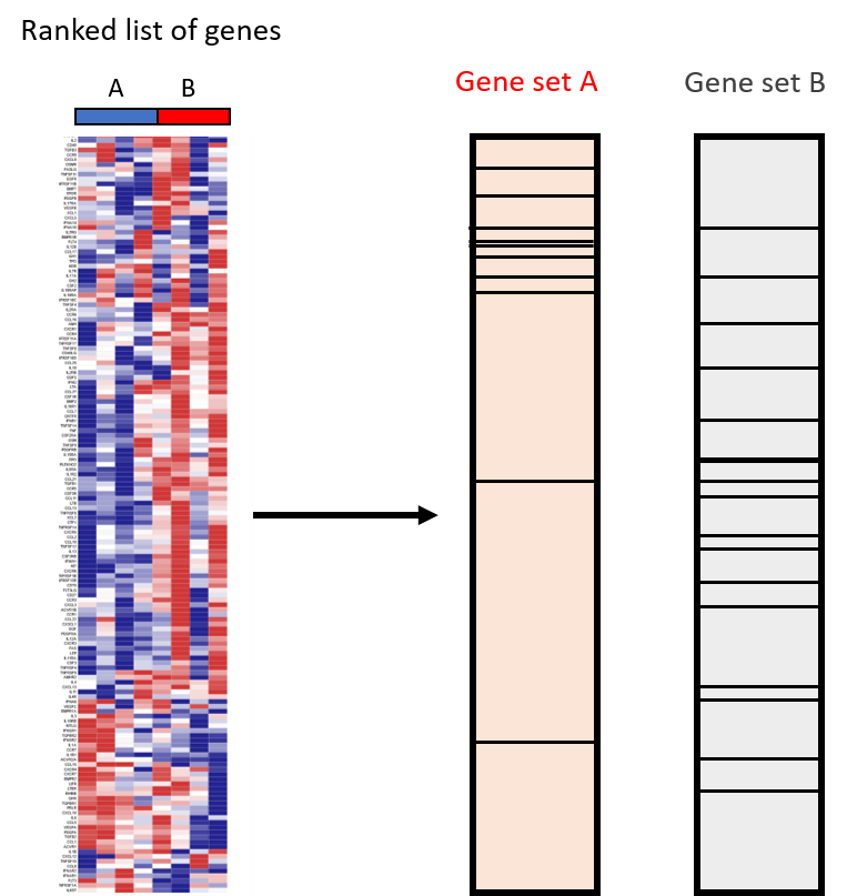
GSEA is a statistical method that determines whether a predefined gene set (GO, KEGG, etc) demonstrates statistically
significant difference between two groups. Taking as input a list of ranked genes and a gene set, it looks at whether the
genes from the gene set are randomly distributed in the ranked list or significantly enriched in the top and bottom
extremes of the ranked list. In the following schema, the gene set A is significantly enriched, while gene set B
represents a case where the genes are more randomly distributed. In contrast to ORA, GSEA can
detect weakly coordinated changes of gene expression in sets of functionally related genes because it is not limited
by the issue of losing information when setting a threshold.
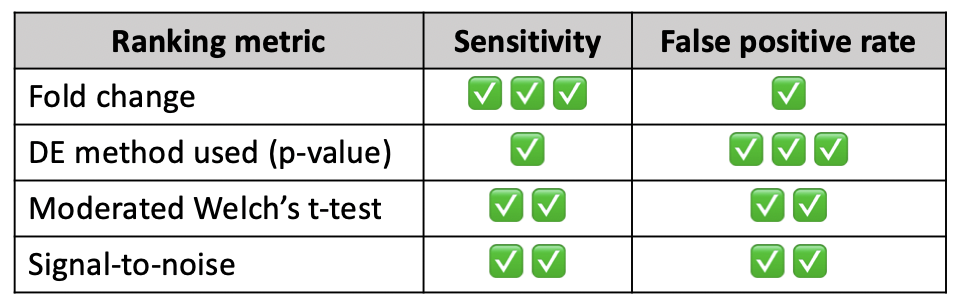
Ranking the list of genes to be analyzed by GSEA is a critical step that can greatly influence the result. Many ranking
metrics are present in the literature and there is no consensus on which is best to use. NetworkAnalyst offers four different
methods. Rank based on DE method used and Fold change are the most intuitive, ranking genes according to their
p-values and fold changes with respect to the primary metadata factor. Moderated Welch's t-test (MWT) and signal-to-noise
ratio (S2N) are two other metrics that have been found to perform well with a low computational load. MWT is a version of
the t-test that allows for unequal variance between groups, and S2N is the difference between the mean expression divided by
the sum of the expression standard deviation for two phenotype groups.
Please note the above gene ranking methods are not applicable to meta-analysis. Instead, the genes are ranked based on the summary statistic obtained
from the previous meta-analysis (combine p-value, effect-size or direct merging). Results obtained from vote count can not be used to perform GSEA.
A recent publication compared different ranking metrics using 28 benchmark datasets and scored each one based on their sensitivity
and false positive rate, summarized in the table below for the four metrics supported by
NetworkAnalyst. While all metrics are widely accepted, you should choose based on how important the sensitivity/false positive
rate is to your analysis. For more details on how the sensitivity and false positive rate were determined,
refer to the original
publication.
The enrichment score is the main output of GSEA. It represents the number of genes in the gene set that are over-represented
at the extremes on the ranked list (most up or down regulated). It is the maximum deviation from zero encountered during
the random walk that goes through the ranked list.
GSEA requires an entire profile of gene expression values, and so it is only available after data processing and differential
analysis of uploaded gene expression table(s) in the GSEA Enrichment Network and GSEA Heatmap Clustering tools.
ORA is more flexible since it only requires a list of genes of interest. In addition to the stand-alone ORA Enrichment
Network and ORA Heatmap Clustering tools, ORA can be performed on subsets of genes identified in volcano plots,
network modules, sections of Venn diagrams and chord diagrams, and the focus view of any heatmap. The GSEA and ORA
enrichment networks are described in more detail in the following FAQ section.
Yes, after you have performed functional enrichment analysis, the significant gene sets will be displayed in
a table. By double clicking on a gene set name, all members will be displayed on the focus view
(heatmap analysis), as highlighted node(s) within the current network (network analysis/enrichment network), as highlighted
points in the volcano plot, or as highlighted chords in the chord diagram.
Enrichment networks are a good way of visualizing the output from enrichment analysis when there are many significant results.
Enriched gene sets are displayed in network form, where gene sets with overlapping genes are connected by edges. This groups
functionally similar gene sets together, which can be easier to interpret than a list of enriched gene sets in tabular form.
Enrichment networks are particularly useful for nested gene sets, such as in the Gene Ontology.
Gene sets are represented by the nodes that are automatically generated in the default view. The nodes are coloured according
to their enrichment score (GSEA) or p-value (ORA) from the results table. The size of the node corresponds to the number
of genes from that gene set that are on the analyzed gene list. The smaller nodes correspond to individual genes, and they
are coloured according to their fold change. More details on how to manipulate the appearance of the network can be found
in the "Network Visualization" section.
Gene set nodes are considered "meta-nodes" because double-clicking them reveals smaller nodes that correspond to the
individual genes belonging to that gene set from the analyzed gene list. There will be an edge between the individual gene
and any enriched gene set that they are a part of, so you can easily see the which genes are shared between sets. The
hierarchical organization of meta-nodes allows users to customize the level of detail represented by an enrichment network.
A bipartite network displays nodes for all gene sets and individual genes. The same network could be generated from the default
enrichment network view by double-clicking each gene set node. Bipartite networks are appropriate when there are a smaller
number of enriched gene sets.
There are two options for determining whether an edge is drawn between two gene sets. The overlap coefficient (OC)
is calculated as the overlap of two gene sets divided by the size of the smaller set. The Jaccard index (JI)
is the overlap of two gene sets divided by the size of their union. The JI is more applicable when gene sets have a
relatively similar size, such as KEGG pathways or PANTHER GO slims. The OC is better at detecting parent-child relationships
within hierarchically organized gene sets, such as the full Gene Ontology.
To increase the size of a gene set node, double-click on the name of the gene set in the results table on the right hand
side. Each time the gene set name is double-clicked, the size will increase. Since the appearance of labels depends on the
size of the node, this is a way too add labels to specific nodes in the network.
If there are a subset of enriched gene sets that are of particular interest, you can visualize them separately from the
rest of the network by extracting them. Select the gene sets from the "Result Table" panel and click the "Extract" button
at the top left corner. If you want to see the detailed connections between a few gene sets (shared individual genes), this
can be an effective way of simplifying the network so that these details are easier to visualize and interpret.
 icon on the left tool bar in the network view window. Note, the operation is computationally
expensive, so you will have to wait for ~20 seconds for the extracted network to return.
The returned network will be named as "moduleX" and is available in the "Network Explorer"
panel on the top-left of the page for future reference.
icon on the left tool bar in the network view window. Note, the operation is computationally
expensive, so you will have to wait for ~20 seconds for the extracted network to return.
The returned network will be named as "moduleX" and is available in the "Network Explorer"
panel on the top-left of the page for future reference.